y+ in CFD Reports: Why the First Cell Decides the Wall Answer
y+ says which part of the boundary layer the first CFD cell sits in, and every wall treatment assumes an answer. I ran a 500 mm air duct in OpenFOAM five ways: the same wall-function mesh moved from y+ 29 to y+ 10 when the flow dropped from 10 to 3 m/s, and wall functions on a y+ 1 mesh gave 164% of the correlation's wall shear. I set out what I ask to see in a report.
When I review a CFD report, one of the first things I look for is a contour of y+ on the walls. It is rarely there. The velocity contours are there, and somewhere in the text there is a line saying the mesh was "refined near the walls". Yet the number that tells me whether the wall shear or the heat transfer coefficient can be trusted is missing.
y+ is the distance of the first cell from the wall, written in wall units: y+ = y·uτ/ν, where uτ is the friction velocity. It is not a quality score where smaller is better. It says which part of the boundary layer the first cell sits in, and every wall treatment in a CFD code assumes a particular answer to that question.
1. The boundary layer has three zones, and the wall models know only two
Near a smooth wall, the textbooks split the flow into a viscous sublayer below y+ of about 5, a log layer above about 30, and a buffer layer in between where neither simple law holds (Pope, Turbulent Flows, chapter 7). Either the mesh resolves the sublayer, with the first cell at y+ around 1 and a model built for it, or the first cell sits in the log layer and a wall function bridges the gap.
The ANSYS Fluent Theory Guide (section 4.12.2) is clear about this. Its log law uses a von Kármán constant of 0.4187 and E of 9.793, it notes that the log law is valid for y* between 30 and 300, and the code switches from the linear relation to the log law at y* = 11.225. For the enhanced wall treatment (section 4.12.4), resolving the sublayer typically means a first node at y+ ≈ 1. OpenFOAM's standard wall functions use the same form with κ = 0.41 and E = 9.8.
Taken alone, the wall law misreads the shear badly in the buffer layer. I compared the standard wall function with a reference profile through all three zones (Spalding's composite law, same constants) and asked what wall shear it would infer from the velocity at a first cell placed at a given y+.

Wall law on its own: shear inferred by a standard wall function (Fluent constants) from the velocity of a reference Spalding profile, equilibrium boundary layer, y* taken equal to y+. Computed for this article.
Read at a single point, the error reaches about 26% low near y+ 13. A real solver does not work that way, though. The wall function and the turbulence model are solved together with the flow, and the profile adjusts. So I ran the case.
2. The same duct in OpenFOAM, five ways
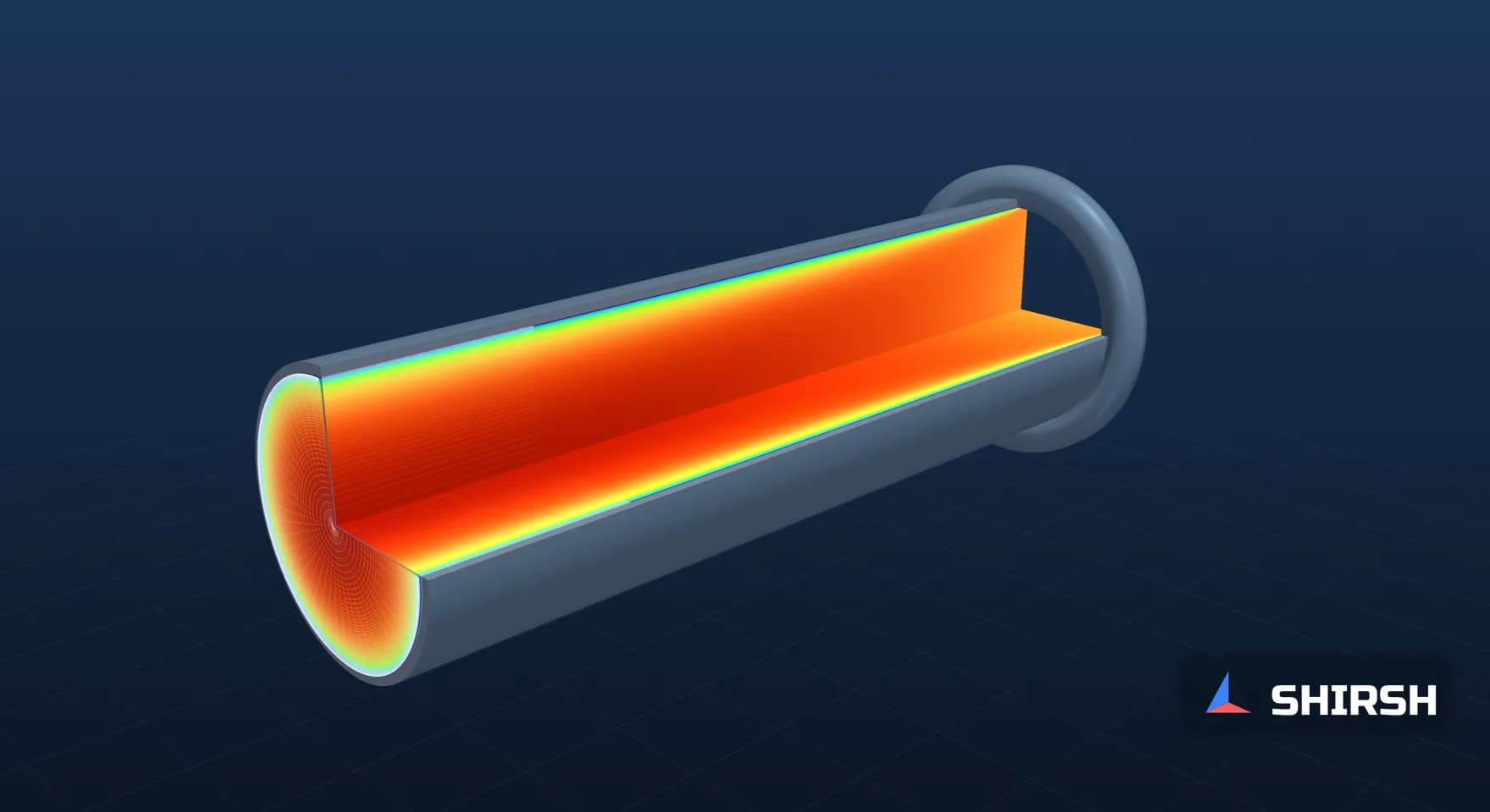
The model is a straight 500 mm round duct carrying air, 30 diameters long, with a uniform inlet, run as an axisymmetric wedge in OpenFOAM's simpleFoam. Two meshes were built for it. One has 90 radial cells with a first cell of 0.0718 mm, sized for y+ ≈ 1 at 10 m/s. The other has 22 radial cells with a first cell of 2.153 mm, sized for y+ ≈ 30. Both first-cell sizes come from the Petukhov smooth-pipe friction factor, which also gives the reference wall shear used below.

Pre-processing: boundary conditions and the near-wall zone of the two meshes, drawn from the actual grading used in the runs.
Cases A and D use the SST model on the fine mesh at 10 and 3 m/s. Cases B and C use k-ε with standard wall functions on the coarse mesh at the same two speeds. Case E is the common mistake: k-ε with standard wall functions on the fine mesh. All cases converged, and the wall shear at x/D = 28 agrees within 3% with the shear backed out of the pressure gradient over x/D 20 to 28.

Post-processing: axial velocity over the duct length for cases A, B and C. The development looks much the same in all three, which is why a contour plot alone says little about the wall.

Still from the 3D streamline animation of cases A to E, built from the computed mean flow (pipe length drawn compressed). The full animation is available as a video.
Case | Model and mesh | Speed, m/s | First-cell y+ at x/D 28 | Wall shear, % of Petukhov | Pressure gradient, Pa/m |
|---|---|---|---|---|---|
A | SST, fine mesh | 10 | 0.97 | 93.4 | 1.60 |
B | k-ε + wall function, coarse mesh | 10 | 29.35 | 95.7 | 1.64 |
E | k-ε + wall function, fine mesh | 10 | 1.28 | 164.4 | 2.73 |
D | SST, fine mesh | 3 | 0.33 | 97.6 | 0.19 |
C | k-ε + wall function, coarse mesh | 3 | 10.32 | 103.4 | 0.20 |

Post-processing: velocity profiles in wall units. Open squares mark the first cell of each mesh.

Post-processing: first-cell y+ along the wall, and wall shear for every case.
Three things come out of it. The coupled buffer-layer error in case C is about 6% against the resolved run D, far smaller than the single-point figure above, and it went the other way, high instead of low. Wall functions on a mesh that is too fine are much worse: case E reports 1.76 times the wall shear of case A and 1.71 times its pressure gradient, from a mesh that looks better on paper. The correlation itself sits a few percent from every model, so the reference carries its own scatter too.
3. The same mesh, a different flow rate
y+ depends on the flow, so a mesh that is right at one operating point can be wrong at another without a single cell changing. The hand estimate said the 2.153 mm cell would drop from y+ 30 at 10 m/s to y+ 10.15 at 3 m/s. The run gave 29.35 and 10.32. Case B reads 95.7% of the correlation and case C 103.4%, so the same model on the same mesh moved by about 8 points between two operating points of one duct.
Liquids make the cells smaller still: water at 25 °C in a 25 mm pipe at 1 m/s needs a 0.98 mm first cell for y+ 30 and 0.033 mm for y+ 1.
4. Heat transfer is less forgiving
A thermal wall function bridges the same gap with its own law. When the purpose of a study is a surface temperature or a heat transfer coefficient, I prefer the near-wall region resolved, with y+ around 1 and a wall treatment built for it, such as the enhanced wall treatment in ANSYS Fluent, SST with automatic wall treatment in ANSYS CFX, or a low-Reynolds treatment in OpenFOAM. Case E is the warning: a fine mesh is only right with a model that expects it.
5. What I ask for in a report
A y+ contour on the walls that carry the answer, with the range shown, for every operating point that is reported. An area-weighted average hides the cells that matter, because y+ wanders furthest from its target in separation and stagnation zones.
A line naming the turbulence model and wall treatment and the y+ range they were built for, next to the range the mesh actually achieved. If the two do not overlap on the walls that matter, I want to see why the result is still usable.
For wall-driven quantities such as pressure drop or heat transfer coefficient, a near-wall sensitivity run, either a second inflation layer stack or a second wall treatment, and a comparison with a correlation where one exists. If the quantity the decision rests on moves by less than the margin in the decision, the question can be closed in one sentence.
Where Shirsh fits
At Shirsh Technosolutions we run CFD in ANSYS Fluent, ANSYS CFX and OpenFOAM, with near-wall meshes set for the wall treatment and the operating points the study has to cover, and we review CFD models and reports prepared by others. If a pressure drop or a heat transfer result in one of your reports depends on the wall, please get in touch and we can look at it together.
References: ANSYS FLUENT 12.0 Theory Guide (2009), section 4.12.2 Standard Wall Functions (κ = 0.4187, E = 9.793; log law valid for 30 < y* < 300; log law employed for y* > 11.225, linear relation below) and section 4.12.4 Enhanced Wall Treatment (first near-wall node typically at y+ ≈ 1). S.B. Pope, Turbulent Flows, Cambridge University Press, 2000, chapter 7. D.B. Spalding, A single formula for the law of the wall, Journal of Applied Mechanics 28 (1961) 455-458. Petukhov friction factor f = (0.790 ln Re − 1.64)⁻² for smooth tubes. Worked check and CFD computed for this article on 21 November 2026: wall-law check with Spalding's law (κ = 0.4187, B = 5.449) as reference; OpenFOAM v1912 simpleFoam, axisymmetric 2.5° wedge, D 0.5 m, L 15 m, air ν = 1.51e-5 m²/s, uniform inlet with 5% turbulence intensity; mesh 300 × 90 cells (first cell 0.0718 mm) and 300 × 22 cells (first cell 2.153 mm); kOmegaSST with nutLowReWallFunction, kEpsilon with nutkWallFunction and epsilonWallFunction (κ 0.41, E 9.8); results at x/D = 28, pressure gradient over x/D 20 to 28 with ρ = 1.204 kg/m³. Generic geometry; not any project.
Related case studies
Want to Apply This to Your Product?
Our engineers can help you implement these techniques on your specific components and assemblies.
Get insights like this in your inbox
Engineering deep-dives, simulation tips, and industry analysis. No spam, unsubscribe any time.