Car Park Ventilation: Why CO Sensors Miss the Moving Dead Zones

A basement car park is usually handed over with a ventilation report that gives an air change rate and a sensor layout that shows CO detectors spaced along the driving aisles. Both can be correct and the car park can still have corners where exhaust gas sits for a long time. The reason is simple. The rate tells you how much air leaves the building. It says nothing about the route that air takes, and the route changes every time a jet fan stops or the extract drops to its low speed.

This article works through a small OpenFOAM study of a generic single-level basement. It shows where the stale air collects with extract fans alone, what four jet fans change, how one fan out of service moves the problem, and what six ordinary aisle sensors actually see in each case.

1. What the codes ask for, and what they leave to the designer

Car park ventilation codes mostly set a quantity. UK Approved Document F (2010 edition, as summarised in 2012 by CIBSE Journal and by Colt) sets the CO limits at 30 ppm averaged over eight hours and 90 ppm over 15 minutes, and suggests six air changes per hour for normal operation. Approved Document B asks for at least 10 air changes per hour from a mechanical system under fire conditions. ASHRAE Standard 62.1-2016, Table 6.5, gives a minimum exhaust rate of 0.75 cfm/ft² (3.8 L/s per m² of floor) for parking garages, and the ASHRAE Applications Handbook (2015), section 15.20, recommends varying the airflow with CO level to save energy where local codes allow it. The Minnesota Mechanical Code (2009), section 404.1, carries the same 0.75 cfm/ft² and requires CO and NO2 detectors that activate the ventilation at 25 ppm CO or 3 ppm NO2.

In India, the Unified Building Bye Laws 2016 (clause 8.4.5 h) send the designer to NBC 2016 Part 4 for the air change rate in fire mode and to Part 8, Section 3 for normal operation.

None of these documents says where the detectors should go or checks that the air reaches every part of the floor. That is left to the designer, and it is where CFD earns its place.

2. The worked example

The model is a generic basement, not any particular building: 48 m long, 32 m wide and 3.0 m clear height, a volume of 4,608 m³. Parked cars fill three bands 40 m long, a 5 m row along each long wall and a 10 m double row in the middle, modelled as high-resistance porous blocks 1.5 m tall. That leaves two 6 m driving aisles along the length and two 4 m cross aisles at the ends. Make-up air enters through a 6 m x 3 m ramp opening at the west end of aisle 1. The extract grille is 6 m x 1.2 m, high on the east wall at the end of aisle 2, so the air has to cross the whole floor diagonally.

At six air changes per hour the extract is 7.68 m³/s, which gives a nominal time constant of 600 s (10 minutes). For comparison, the ASHRAE floor-area rate for this 1,536 m² floor would be 5.85 m³/s, or 4.57 air changes per hour at this height.

Four jet fans, J1 to J4, hang at 2.4 to 2.7 m on the centrelines of the two aisles at 12 m and 30 m from the west wall, all blowing east towards the extract. Each is a 50 N thrust source, a typical size chosen for this example. Six CO sensors, S1 to S6, sit at 1.5 m on the aisle centrelines at 8, 24 and 40 m, which is the kind of even layout often drawn at tender stage.

Figure 1. Worked example in plan. Make-up air comes in through the ramp (green), leaves through the extract grille (red). Jet fans J1 to J4 blow east; triangles mark the six sensors at 1.5 m.

We solved steady incompressible flow with OpenFOAM (simpleFoam, k-epsilon, wall functions) on a uniform hexahedral mesh of 61,440 cells, 0.5 m in plan and 0.3 m in height. Vehicle exhaust is represented by a uniform passive emission in the bottom 0.3 m of all aisles. Two passive scalars were then solved on each flow field: the local mean age of air, and the exhaust concentration. Concentration is reported as C/Cmix, where Cmix is the value the whole car park would have if the extract air were perfectly mixed. A value of 1.0 means "as good as perfect mixing"; 3.0 means three times worse. Because the scalar equations are linear, these ratios hold for any emission rate, so they translate directly into ppm once a design emission is chosen.

Four cases were run:

• Case A: extract only at 6 ACH, jet fans off.

• Case B: 6 ACH with all four jet fans running.

• Case C: as B with J3, the upstream fan in aisle 2, out of service.

• Case D: extract at low speed, 3 ACH (3.84 m³/s), with all four jet fans running.

3. Results at a glance

Table 1. Results at 1.5 m over the driving and cross aisles. Each case is normalised by its own nominal time constant and its own Cmix; case D has half the airflow, so its nominal time constant is 20 minutes and its Cmix is twice that of the 6 ACH cases. Air change effectiveness is the nominal time constant divided by twice the mean age, so 50% corresponds to perfect mixing.

4. Case A: the rate is right and half the aisles are still

With the extract alone, the air takes the shortest route. It enters at the ramp, runs as a fast stream along aisle 1, turns at the east end and leaves. Aisle 1 near the ramp is the cleanest place in the car park, which is why S1 reads 0.00 there. Everything away from that stream is fed only by slow recirculation. At 1.5 m, 46.2% of the aisle area moves at less than 0.1 m/s, and the mean age of air is 1.86 times the nominal value, so the car park behaves much worse than a well-mixed room even though the extract meets the 6 ACH figure exactly.

The worst point at sensor height, 6.88 times Cmix, is in the west cross aisle in the corner between the ramp opening and the south wall. It is a pocket that the incoming stream sweeps past and never enters. The highest of the six sensors is S5 in the middle of aisle 2 at 2.36. If S5 were set to switch the fans at 25 ppm, the same steady pattern would put that corner at 72.8 ppm.

5. Case B: jet fans fix the route

Four jet fans with the same extract change the picture completely. The fans in aisle 2 pull air in from the west cross aisle and drive it to the extract, so the second aisle becomes a flow path of its own. Air change effectiveness rises from 26.9% to 60.7%, which means the jets have turned a short-circuiting layout into one that slightly beats perfect mixing. The share of slow aisle area falls from 46.2% to 7.9%, and the worst aisle point falls from 6.88 to 1.72.

The dead zone has not vanished, though. It has moved. In case A it was in the south-west corner beside the ramp. In case B it sits further north in the west cross aisle, opposite the west end of the double row, where the air turning into aisle 2 leaves a slow region against the parked cars. None of the six sensors is in a cross aisle. The highest reading is 1.19 at S4, so a 25 ppm setpoint at S4 would correspond to about 36.2 ppm at the worst point.

Figure 2. CO at 1.5 m relative to the well-mixed value, aisles only (parked-car bands in grey). The green ring marks the worst aisle point in each case; triangles are the six sensors. The stale area moves from the ramp corner (A) to the west cross aisle (B, C, D) and spreads along aisle 2 when J3 is off (C).

6. Case C: one fan off and the pattern shifts again

In a real car park a jet fan is sometimes out of service, whether it has tripped or been isolated for maintenance. Case C turns off J3, the upstream fan in aisle 2. The extract and the other three fans are unchanged.

The west half of aisle 2 loses its driving jet, and the air there slows down. The share of aisle area below 0.1 m/s rises from 7.9% to 29.6%. Mean C/Cmix in aisle 2 goes from 1.05 to 1.27, and in the west cross aisle from 0.91 to 1.05. The worst aisle point rises from 1.72 to 2.69 and stays in the west cross aisle, a little south of where it was in case B. Air change effectiveness drops from 60.7% to 44.1%.

S4 is still the highest sensor, but it only rises from 1.19 to 1.38. The gap between what the sensors report and what the worst point sees has grown. At a 25 ppm setpoint on S4, the worst point would now be at 49.0 ppm. In other words, the sensor layout that looked adequate for case B is noticeably less adequate the day one fan is out.

Figure 3. What the six sensors read, against the worst aisle point at the same height. Case A shows the largest gap; case C shows how a single fan out of service widens it again.

7. Case D: low speed keeps the pattern and doubles the level

Many car parks run the extract at low speed most of the day and ramp it up on CO. Case D halves the extract to 3 ACH and keeps all four jet fans at full thrust. Normalised by its own Cmix, the pattern is very close to case B: air change effectiveness 59.5%, worst point 1.67 in the west cross aisle, highest sensor 1.08 at S4. The jets dominate the flow, so the route barely changes when the extract slows.

The level does change. With half the air, Cmix doubles, so in terms of the 6 ACH well-mixed value the aisle mean is 1.66 and S4 reads 2.16. This is the behaviour CO control relies on, and it works here because the jet fans keep the route intact. Had the jets been staged down with the extract, case A is the reminder of what an unassisted route looks like.

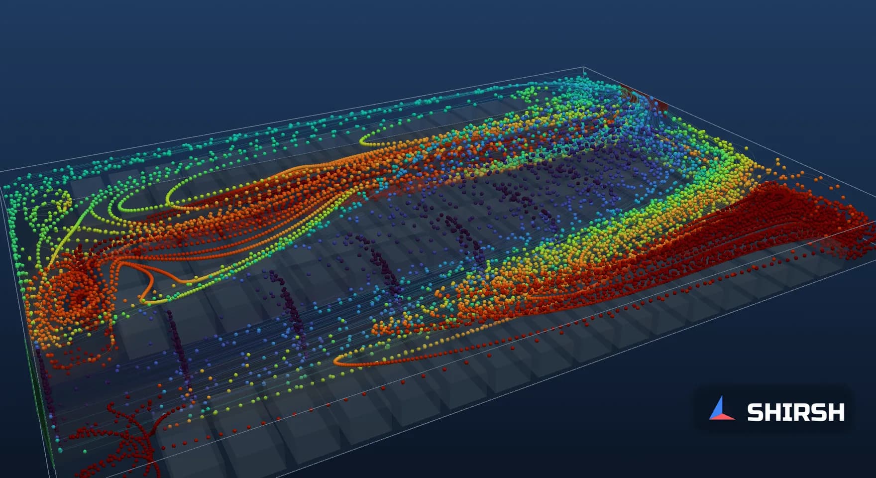
Figure 4. Streamlines of the converged flow in case C, coloured by CO relative to the well-mixed value, with the six sensor readings and the worst aisle point. Frame from the 3D streamline animation of all four cases; it illustrates the steady flow field, not a transient result.

8. Mesh check, convergence and limits

Case B was re-run on a 276,480-cell mesh (1/3 m in plan, 0.15 m in height), started from the coarse solution. Air change effectiveness moved from 60.7% to 60.1%, mean C/Cmix in the aisles from 0.79 to 0.81 and the S4 reading from 1.19 to 1.24. The worst aisle point rose from 1.72 to 1.91 and stayed in the west cross aisle, about 6 m further south. The share of slow aisle area moved from 7.9% to 14.2%, so that figure should be read as a trend between cases rather than a precise value. Local peaks are always the most mesh-sensitive number in a study like this, which is a good reason not to place a sensor on the strength of a single coarse run.

Cases B, C and D converged to residuals of 1e-5 in pressure, and their aisle results did not change between iteration 2000 and the final iteration. Case A did not settle to a steady state; the slow recirculation keeps wandering, as it often does in a weakly driven space. Its flow field was therefore averaged over ten snapshots between iterations 2600 and 3500. The two halves of that window gave air change effectiveness of 26.6% and 27.1%, a worst point of 6.86 and 6.90, and S5 readings of 2.30 and 2.44.

The model has clear limits. Cars are porous blocks rather than individual vehicles, there are no columns, beams, ducts or ramps inside the floor, and the emission is spread evenly over the aisles rather than following real traffic. Buoyancy from warm exhaust and hot engines is left out, and so is wind acting on the ramp opening. Moving cars stir the air in ways a steady model cannot show. The numbers belong to this model. What carries over is the method, and the observation that the stale zone moves whenever the driving jets change.

9. What to ask for in a car park ventilation study

The useful evidence is short. The study should show the flow route from the make-up openings to the extract in plan, at sensor height, for each operating mode the controls can produce: extract only, jet fans running, low-speed extract and at least one fan out of service. It should report the worst aisle point at 1.5 m for each mode and where it sits, and compare it with what the proposed detectors would read. Cross aisles, corners beside ramps and the ends of double rows are the first places to look, because the main jets pass them by.

Sensor positions then come from those maps rather than from an even grid. In this example, a seventh detector in the west cross aisle, 2 m from the wall and 13 m from the south wall, would have read 1.36, 1.48 and 1.43 in cases B, C and D, higher than any of the six aisle sensors. In case A it would have read 2.20, still short of S5, because the worst corner there sits right beside the ramp. No single position covers every mode, which is the argument for checking each one.

Where Shirsh fits

At Shirsh Technosolutions we carry out CFD studies of basement and multi-level car parks with ANSYS Fluent and OpenFOAM, covering normal ventilation, jet fan layouts, CO sensor placement, fan failure cases and smoke clearance in fire mode. If you are laying out a car park ventilation system or checking one that does not seem to clear properly, please get in touch.

References
Approved Document F (2010) and Approved Document B, as summarised in R. Brooks and S. Elves, "On the right track", CIBSE Journal, July 2012 (CO limits, fire-mode air change rate), and in Colt, "How much ventilation is needed to make car parks safe?", October 2012 (six air changes per hour).
ASHRAE Standard 62.1-2016, Table 6.5, and ASHRAE Interpretation IC 62.1-2016-5 (2018), which cites the ASHRAE Applications Handbook (2015), section 15.20.
Minnesota Mechanical Code (2009), section 404.1 Enclosed parking garages, as quoted in MNOSHA Instruction STD 5-1.2B (2024).
Unified Building Bye Laws 2016, clause 8.4.5 h, as tabulated in HUDCO Shelter, October 2022 (reference to NBC 2016 Part 4 and Part 8, Section 3).
Worked example: OpenFOAM v1912 runs of cases A to D and the case B mesh check, computed for this article on 6 November 2026. Generic basement; not any project.